Neural Network and Back Propagation Algorithm

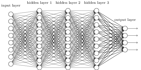
Neural networks are typically organized in layers. Layers are made up of a number of interconnected nodes which contain an activation function $h_\theta(z)$. Patterns $\mathbf{x}$ are presented to the network via the input layer, which communicates to one or more hidden layers where the actual processing is done via a system of weighted connections $\mathbf{\Theta}$. The hidden layers then link to an output layer where the predict answer $\mathbf{y}^{pred}$ is output as shown in the graphic below.

An artificial neural network with 3 hidden layers.

Math Model

Here, we use the sigmoid function as activation function:

$$h(z)=\frac{1}{1+e^{-z}},$$

which has a convenient derivative of:

$$h'(z)=h(z)(1-h(z)).$$

We assume there are L layers of neural networks and label nodes of layer $i$ as $\mathbf{a}^{(i)}$ and call them “activation units”. The output of the $i^{th}$ layer is the input of the $i+1^{th}$ layer. In the input layer,

$$\mathbf{a}^{(0)}:=\begin{bmatrix}1 \\ \mathbf{x}\end{bmatrix};$$

and in the output layer,

$$\mathbf{a}^{(L)}:=\mathbf{y}^{pred}.$$

$\mathbf{a}^{(i)}$ can be solved in a feed-forward manner, as:

$$\begin{align*} \mathbf{z}^{(i)}&=\theta^{(i)}\cdot\begin{bmatrix}1 \\ \mathbf{a}^{(i-1)}\end{bmatrix}\\ \mathbf{a}^{(i)}&=h(z^{(i)}) \end{align*}.$$

Given the trainning set $\{ (\mathbf{x}_1, \mathbf{y}_1), (\mathbf{x}_2, \mathbf{y}_2), \cdots, (\mathbf{x}_M, \mathbf{y}_M)\}$, the cost function for this neural network can be written as:

$$J(\Theta)=-\frac{1}{M}\sum_{t=1}^{M}(\mathbf{y}_t^{T}\cdot\log(\mathbf{y}_t^{pred})+(1-\mathbf{y}_t)^{T}\cdot\log(1-\mathbf{y}_t^{pred}))$$

To ease the derivation, the above formulations can be written in indicial notation, as:

$$\begin{align*} z^{(l)}_{i}&=\theta^{(l)}_{ij}a^{(l-1)}_{j},\\ z^{(l)}_{0}&=\sum\theta^{(l)}_{0j},\\ J(\Theta)&=-\frac{1}{M}(\mathbf{y}_{t,k}\log(\mathbf{y}_{t,k}^{pred})+(1-\mathbf{y}_{t,k})\log(1-\mathbf{y}_{t,k}^{pred})). \end{align*}$$

Following the Einstein summation convention, the repeated free indices are implicitly summed over their range.

The goal of the neural network trainning process is to find the weights $\Theta^{(i)}$ for $i\in\{1,2,\dots, L\}$ such that the cost function approach its maximum for all trianning set. In order to find the maximum by using the gradient descent method, we need to evaluate $J(\Theta)$ as well as the gradient $\frac{\partial{J}}{\partial{\theta^{(l)}_{ij}}}$.

Back propagation Algorithm

Back propagation is a method used in artificial neural networks to calculate the gradients of cost function. Indeed, back propagation is nothing but the chain rule for solving the derivative of compound functions. To demonstrate how it works, we start from the gradient of weights of the output layer ($l=L$):

$$\frac{\partial{J}}{\partial{\theta^{(L)}_{ij}}}=\frac{1}{M}\left({\frac{a^{(L)}_{t,k}-y_{t,k}}{a^{(L)}_{t,k}\left(1-a^{(L)}_{t,k}\right)}}\right)\frac{\partial{}a^{(L)}_{t,k}}{\partial{\theta^{(L)}_{ij}}},$$

where

$$\frac{\partial{}a^{(L)}_{t,k}}{\partial{\theta^{(L)}_{ij}}} = \left({a^{(L)}_{t,k}\left(1-a^{(L)}_{t,k}\right)}\right)\frac{\partial{}z^{(L)}_{t,k}}{\partial{\theta^{(L)}_{ij}}},$$

with

$$\frac{\partial{}z^{(L)}_{t,k}}{\partial{\theta^{(L)}_{ij}}} = \delta_{ik}\delta_{jl}a^{(L-1)}_{t,l} = \delta_{ik}a^{(L-1)}_{t,j},$$

where $\delta_{ij}$ is the Kronecker delta, with the property:

$$\delta_{ij}= \begin{cases} 0,\quad{i\neq{j}} \\ 1,\quad{i={j}} \end{cases}.$$

Hence,

$$\begin{align*} \frac{\partial{J}}{\partial{\theta^{(L)}_{ij}}}&=\frac{1}{M}\left({a^{(L)}_{t,k}-y_{t,k}}\right)\delta_{ik}a^{(L-1)}_{t,j}\\ &=\frac{1}{M}\left({a^{(L)}_{t,i}-y_{t,i}}\right)a^{(L-1)}_{t,j}. \end{align*}$$

The above formulation is indeed the gradient for logistic regression without regularization term. Now, let’s move one step ahead and find the derivatives of the cost function $J$ w.r.t. the weights $\theta^{(L-1)}_{ij}$. By the chain rule, we can use the formulation we derived above and write:

$$\frac{\partial{J}}{\partial{\theta^{(L-1)}_{ij}}}=\frac{1}{M}\left({a^{(L)}_{t,k}-y_{t,k}}\right)\frac{\partial{}z^{(L)}_{t,k}}{\partial{\theta^{(L-1)}_{ij}}}.$$

From $z_k^{(L)}=\theta_{km}^{(L)}a^{(L-1)}_m$, we have

$$\frac{\partial{}z^{(L)}_{t,k}}{\partial{\theta^{(L-1)}_{ij}}}=\theta_{km}^{(L)}a^{(L-1)}_m\left(1-a^{(L-1)}_m\right)\frac{\partial{}z^{(L-1)}_{t,m}}{\partial{\theta^{(L-1)}_{ij}}}.$$

In the Einstein summation convention, each index can appear at most twice in any term. And the index $m$ above does not indicate summation. Hence, we can define an auxiliary second order tensor

$$\lambda^{(l)}_{ij}=\theta_{ij}^{(l+1)}a^{(l)}_j\left(1-a^{(l)}_j\right).$$

Then,

$$\begin{align*} \frac{\partial{J}}{\partial{\theta^{(L-1)}_{ij}}}&=\frac{1}{M}\left({a^{(L)}_{t,k}-y_{t,k}}\right)\lambda^{(L-1)}_{km}\delta_{mi}\delta_{lj}a^{(L-2)}_{t,l}\\ &=\frac{1}{M}\left({a^{(L)}_{t,k}-y_{t,k}}\right)\lambda^{(L-1)}_{ki}a^{(L-2)}_{t,j} \end{align*}.$$

Following the same pattern, you can derive

$$\frac{\partial{J}}{\partial{\theta^{(L-2)}_{ij}}}=\frac{1}{M}\left({a^{(L)}_{t,k}-y_{t,k}}\right)\lambda^{(L-1)}_{kl}\lambda^{(L-2)}_{li}a^{(L-3)}_{t,j}.$$

By mathematical induction, you may find

$$\frac{\partial{J}}{\partial{\theta^{(l)}_{ij}}}=\frac{1}{M}\left({a^{(L)}_{t,k}-y_{t,k}}\right)\lambda^{(L-1)}_{km}\lambda^{(L-2)}_{mn}\dots\lambda^{(l)}_{pi}a^{(l-1)}_{t,j}, \quad \forall{l=1,2,\dots, L-1}.$$

For the regularized neural network, all you need to do is to add the derivative of the regularization term w.r.t. the corresponding weights, which is a trivial task.